From personal project to industry standard

Introduction added in 2025

When introduced Oklab in 2020, I never expected it to reach as far as it has. In a few years Oklab has, among other things, found its way into:

• Photoshop – Now the default interpolation method for gradients
• Web browsers – Part of CSS Color Level 4 and 5, supported by major browsers
• Game engines – Used in Unity’s gradients and Godot’s color picker
• Open source libraries – Too many to list! For python, I recommend colour.

I developed Oklab in my free time and the results are freely available and open source. Want to support my work? Here are some options:

• I’m available for contracting work in color science, computer graphics, game dev and more.
• I’m an indie game developer making Island Architect, a cozy town building game. Consider sharing and wishlisting. It is of course using Oklab here and there!

Below you find the original blog post introducing Oklab, from 2020.

A perceptual color space for image processing

A perceptual color space is desirable when doing many kinds of image processing. It is useful for things like:

• Turning an image grayscale, while keeping the perceived lightness the same
• Increasing the saturation of colors, while maintaining perceived hue and lightness
• Creating smooth and uniform looking transitions between colors

Unfortunately, as far as I am aware, while there are color spaces that aim to be perceptually uniform, none are without significant drawbacks when used for image processing.

For this reason I have designed a new perceptual color space, designed to be simple to use, while doing a good job at predicting perceived lightness, chroma and hue. It is called the Oklab color space, because it is an OK Lab color space.

Before diving into the details of why a new color space is needed and how it was derived, here is the everything needed to use the color space:

The Oklab color space

A color in Oklab is represented with three coordinates, similar to how CIELAB works, but with better perceptual properties. Oklab uses a D65 whitepoint, since this is what sRGB and other common color spaces use. The three coordinates are:

• $L$ – perceived lightness
• $a$ – how green/red the color is
• $b$ – how blue/yellow the color is

For many operations, $Lab$-coordinates can be used directly, but they can also be transformed into polar form, with the coordinates lightness, chroma and hue, $LCh$:

$C={\sqrt {a^2+b^2}}, \qquad h^{\circ}=\text{atan2}(b,a)$

From $C$ and $h^{\circ}$, $a$ and $b$ can be computed like this:

$a=C\cos(h^{\circ}),\qquad b=C\sin(h^{\circ})$

Lets look at a practical example to see how Oklab performs, before looking at how the $Lab$ coordinates are computed.

Comparing Oklab to HSV

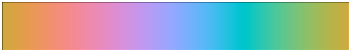
Here’s an Oklab color gradient with varying hue and constant lightness and chroma.

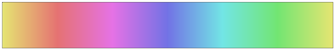
Compare this to a similar plot of a HSV color gradient with varying hue and constant value and saturation (HSV using the sRGB color space).

The gradient is quite uneven and there are clear differences in lightness for different hues. Yellow, magenta and cyan appear much lighter than red and blue.

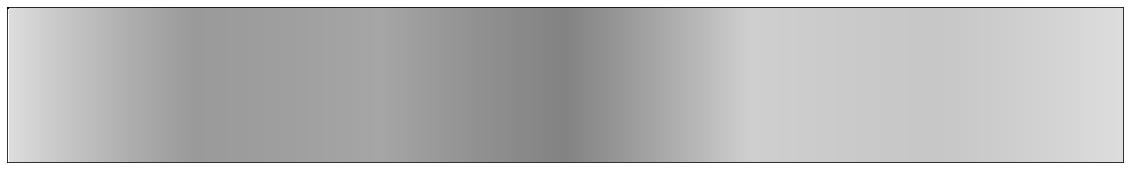
Here is lightness of the HSV plot, as predicted by Oklab:

Implementation

Converting from XYZ to Oklab

Given a color in $XYZ$ coordinates, with a D65 whitepoint and white as Y=1, Oklab coordinates can be computed like this:

First the $XYZ$ coordinates are converted to an approximate cone responses:

$\begin{pmatrix} l \\ m \\ s \end{pmatrix} = \mathbf{M_1} \times \begin{pmatrix} X \\ Y \\ Z \end{pmatrix}$

A non-linearity is applied:

$\begin{pmatrix} l' \\ m' \\ s' \end{pmatrix} = \begin{pmatrix} l^{\frac 1 3} \\ m^{\frac 1 3} \\ s^{\frac 1 3} \end{pmatrix}$

Finally, this is transformed into the $Lab$-coordinates:

$\begin{pmatrix} L \\ a \\ b \end{pmatrix} = \mathbf{M_2} \times \begin{pmatrix} l' \\ m' \\ s' \end{pmatrix}$

with the following values for $\mathbf{M_1}$ and $\mathbf{M_2}$:

$\mathbf{M_1} = \begin{pmatrix} +0.8189330101 & +0.3618667424 & -0.1288597137 \\ +0.0329845436 & +0.9293118715 & +0.0361456387 \\ +0.0482003018 & +0.2643662691 & +0.6338517070 \end{pmatrix}$

$\mathbf{M_2} = \begin{pmatrix} +0.2104542553 & +0.7936177850 & -0.0040720468 \\ +1.9779984951 & -2.4285922050 & +0.4505937099 \\ +0.0259040371 & +0.7827717662 & -0.8086757660 \end{pmatrix}$